What Actually Happens Between Your Prompt and the Next Token?
A deep technical guide to LLM internals, from raw text to token generation, with Python implementations from scratch.
On this page
When you send a prompt to an LLM, it doesn't read your words the way a human does. It doesn't directly understand sentences, look up the next word in a dictionary, or write a response one word at a time.
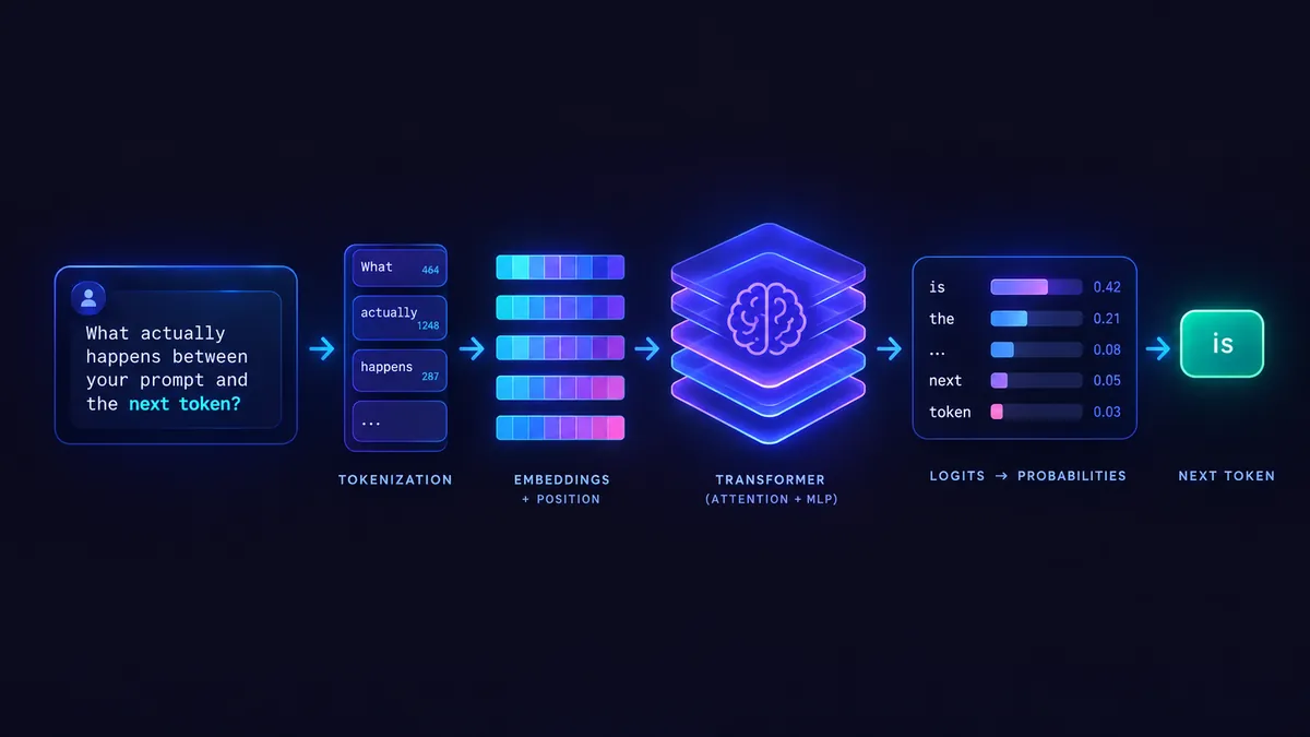
Instead, your prompt passes through a series of computational transformations:
- Text is converted into tokens.
- Tokens are mapped to numerical vectors called embeddings.
- Positional information is incorporated into those representations.
- Transformer layers use attention and neural networks to compute contextual representations.
- The final hidden state is converted into vocabulary-sized logits.
- A sampling or selection strategy chooses the next token.
- The selected token is appended to the sequence, and the process repeats.
All of this happens through numerical operations on tensors, primarily matrix multiplications, attention operations, and nonlinear transformations.
The central idea: an LLM generates text by repeatedly estimating a probability distribution over the next token, conditioned on the tokens already in its context.
Let's follow one prompt through the entire pipeline and implement the important pieces ourselves.
1. The complete journey: prompt to next token
Suppose we send this prompt:
Explain how a database index works in simple terms.
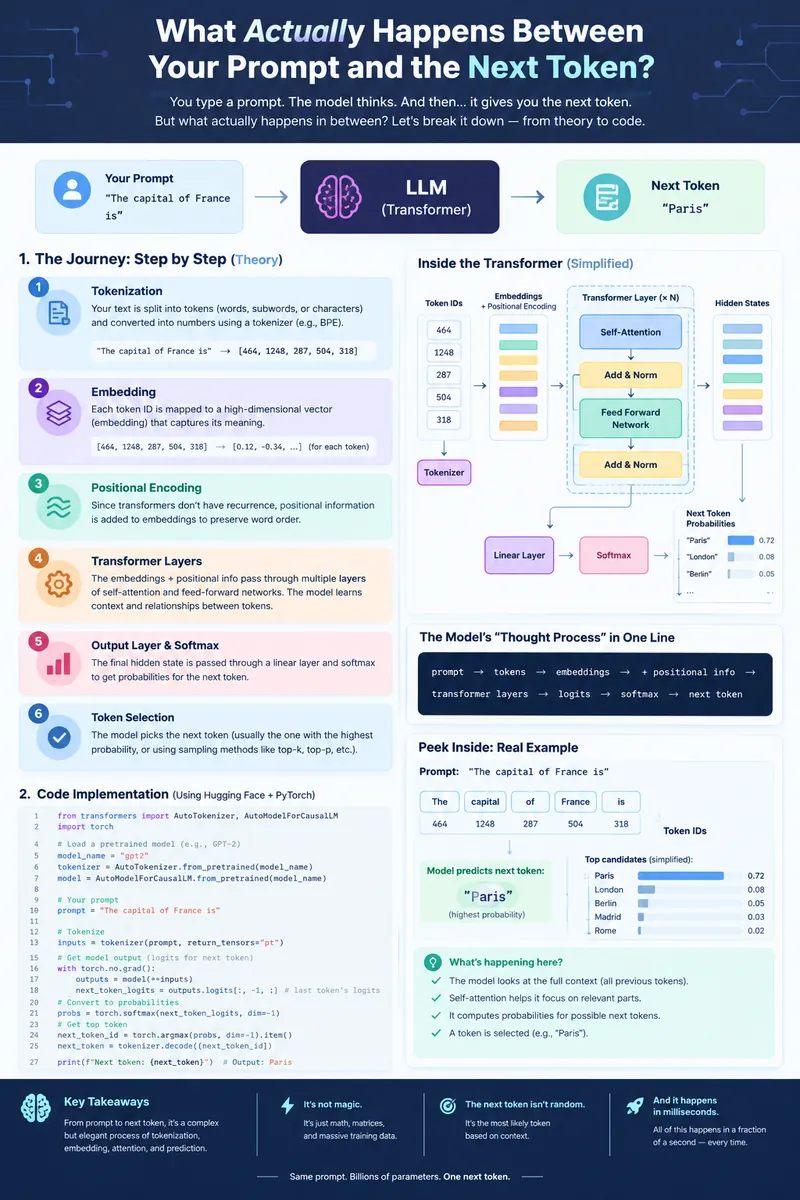
A simplified view of the process looks like this:
- Input promptraw text from the user
- Tokenizationtext → token IDs [4821, 917, 340, ...]
- Embedding + positiontoken IDs → vectors containing learned representations
- *Transformer layers*self-attention + feed-forward + residuals + normalization, repeated across many layers
- Vocabulary projectionfinal hidden state → logits → token probabilities
- Select the next tokengreedy decoding, sampling, or another strategy
- Append token and repeatthe new token becomes part of the context
This is a simplified decoder-only Transformer pipeline. Real systems may also include chat templates, system instructions, tool-routing logic, multimodal inputs, constrained decoding, and serving optimizations.
We will focus on the core text-generation path.
2. Step one: tokenization, converting text into IDs
The model doesn't directly operate on strings such as "database index". It operates on token IDs.
A tokenizer splits text into units from a fixed vocabulary. Depending on the tokenizer, a token might represent:
- A complete word, such as
database - A word fragment, such as
dataorbase - Punctuation, such as
. - Whitespace, or a combination of whitespace and text
- A special token used to mark a message boundary or another control instruction
The important distinction is that tokens are not necessarily words.
For example, a hypothetical tokenizer might convert:
The database is fast.
into:
["The", " database", " is", " fast", "."]The actual tokens depend on the tokenizer and its vocabulary. This example is illustrative, not a claim about any specific model's token IDs.
Each token maps to an integer:
"The"       → 791
" database" → 4821
" is"       → 374
" fast"     → 1290
"."         → 13
These IDs are arbitrary vocabulary indices, not numerical meanings. Token 4821 is not inherently more important or semantically larger than token 374.
2.1 Why not tokenize by splitting on spaces?
Consider:
unbelievable
unbelievably
unbelievable!
A subword tokenizer may reuse some pieces across these strings. This lets a finite vocabulary represent a large variety of words, spellings, and technical terms without requiring every possible word to have its own token.
Tokenization affects:
- The number of tokens in a prompt
- Context-window consumption
- Input and output pricing for token-billed APIs
- How text is represented before it reaches the neural network
2.2 Code: using a real tokenizer
Install the dependencies:
pip install transformers torchUse a publicly available tokenizer for demonstration:
from transformers import AutoTokenizer

model_name = "gpt2"

tokenizer = AutoTokenizer.from_pretrained(model_name)

prompt = "Explain how a database index works."

tokens = tokenizer.tokenize(prompt)
token_ids = tokenizer.encode(prompt)

print("Text:", prompt)
print("Tokens:", tokens)
print("Token IDs:", token_ids)

print("Decoded:", tokenizer.decode(token_ids))
print("Token count:", len(token_ids))
This demonstrates the tokenizer interface using GPT-2's tokenizer. It does not imply that every LLM uses the same vocabulary, tokenization algorithm, or special tokens.
Engineering insight: when debugging a prompt that exceeds the context window, inspect the actual token count instead of estimating from the number of words.
3. Step two: token embeddings, turning IDs into vectors
An integer token ID is useful as an index, but it isn't a representation the Transformer can reason with directly.
The model therefore uses a learned embedding matrix. Suppose the vocabulary contains V tokens and the model's hidden dimension is d. The embedding matrix is:
E ∈ ℝ^(V × d)Each row corresponds to one token's learned vector. If the vocabulary size is V = 50,000 and the hidden dimension is d = 768, then:
E ∈ ℝ^(50000 × 768)A token ID selects one row from this matrix. For example:
Token ID:  4821
Embedding: [0.12, -0.34, 0.81, 0.07, ..., -0.15]
That vector has 768 dimensions in this example.
It is not a dictionary definition or a human-readable semantic record. Its numerical values are learned during training and become useful through their interaction with the model's other learned parameters.
3.1 What do embeddings actually represent?
Embedding dimensions don't generally correspond to clean, individually interpretable properties such as "database", "positive sentiment", or "past tense".
Instead, the representation is distributed across dimensions. The model learns patterns that help it predict tokens across many contexts.
Two tokens used in similar contexts may have related representations, but semantic similarity is not guaranteed simply by looking at their raw embedding vectors.
3.2 Code: inspecting embeddings
import torch
from transformers import AutoModel, AutoTokenizer

model_name = "gpt2"

tokenizer = AutoTokenizer.from_pretrained(model_name)
model = AutoModel.from_pretrained(model_name)
model.eval()

prompt = "Databases need efficient indexes."

inputs = tokenizer(prompt, return_tensors="pt")

with torch.no_grad():
    token_ids = inputs["input_ids"]
    embeddings = model.get_input_embeddings()(token_ids)

print("Token IDs shape:", token_ids.shape)
print("Embedding shape:", embeddings.shape)
print("First token vector:", embeddings[0, 0, :10])
For a prompt with n tokens, the shape is (n, d) (plus a leading batch dimension). In this GPT-2 example, d = 768. The first dimension after the batch represents token positions in the prompt.
Notice that this code accesses the input embeddings only. These vectors are not yet the final contextual representations produced by the Transformer.
4. Step three: positional information, because token order matters
Consider these two sentences:
The engineer reviewed the code.
The code reviewed the engineer.
They contain the same words, but the order changes the meaning.
A Transformer needs information about where tokens occur in a sequence. Otherwise, its attention operation alone would not distinguish the original order.
A common conceptual representation is:
xᵢ = eᵢ + pᵢWhere:
eᵢis the embedding for tokeni.pᵢis the positional representation for positioni.xᵢis the initial representation passed into the Transformer.
This equation describes additive positional encoding, but not every modern Transformer implements position in exactly this way.
4.1 Different approaches to position
| Approach | How it works |
|---|---|
| Sinusoidal positional encoding | Uses deterministic sine and cosine functions at different frequencies. |
| Learned positional embeddings | Learns a vector for each supported position during training. |
| Rotary positional embeddings (RoPE) | Applies position-dependent rotations to query and key vectors in attention. |
| Relative-position methods | Represent positional relationships between tokens rather than relying solely on absolute positions. |
Modern decoder-only models commonly use RoPE or other position-aware mechanisms. GPT-2, used in our examples, uses learned positional embeddings.
4.2 Code: positional embeddings in GPT-2
import torch
from transformers import AutoModel

model = AutoModel.from_pretrained("gpt2")
model.eval()

position_ids = torch.arange(5).unsqueeze(0)

with torch.no_grad():
    position_vectors = model.wpe(position_ids)

print(position_vectors.shape)
Output:
torch.Size([1, 5, 768])This extracts GPT-2's learned positional vectors for five positions.
In GPT-2, token embeddings and positional embeddings are added together before entering the Transformer blocks:
with torch.no_grad():
    token_embeddings = model.wte(token_ids)
    position_embeddings = model.wpe(position_ids)

    initial_hidden_states = token_embeddings + position_embeddings
Here, token_ids must contain five token positions for this exact example to align with position_ids.
The broader lesson is that the Transformer receives numerical representations of both token identity and sequence position.
5. Step four: self-attention, how tokens exchange information
Self-attention is one of the central mechanisms behind a Transformer. At a high level, it allows a token's representation to incorporate information from other tokens in its context.
Consider:
The database rejected the query because it was malformed.
When processing it, the model can use information from earlier tokens to estimate what it refers to.
Attention does not guarantee perfect coreference resolution. It provides a learned mechanism for relating token representations.
5.1 Queries, keys, and values
Each input representation is projected into three vectors:
- Query (Q): what information this position is looking for.
- Key (K): what information this position makes available for matching.
- Value (V): the information contributed if the position receives attention.
These are computational interpretations, not literal questions or labels stored inside the model.
Let the input hidden-state matrix be X ∈ ℝ^(n × d). The projections are:
Q = X·W_Q K = X·W_K V = X·W_VThe projection matrices are learned parameters. For a single attention head with key dimension d_k and value dimension d_v:
W_Q ∈ ℝ^(d × d_k)
W_K ∈ ℝ^(d × d_k)
W_V ∈ ℝ^(d × d_v)
The resulting matrices contain a query, key, and value vector for each token position.
5.2 Calculating attention scores
The model compares each query with the keys of the available positions using dot products:
S = Q·Kᵀ / √d_kThe division by √d_k helps control the scale of the dot products as the key dimension increases. Without appropriate scaling, large dot products can push the softmax function into regions where gradients become very small.
The score matrix S has shape (n, n). Each entry represents the compatibility score between a query position and a key position, before applying the attention mask and softmax.
5.3 Why softmax is needed
Raw attention scores can be positive or negative. Softmax converts each row into normalized weights:
A = softmax(S)For a given query position, these weights sum to one across the allowed key positions. The model then combines the value vectors using those weights:
O = A·VThe output at each position is a weighted combination of information from the available positions.
5.4 Causal masking: preventing future-token leakage
For autoregressive text generation, the model must not use future tokens when predicting the next token.
When processing:
The database uses
the representation at The must not access database or uses through self-attention. The representation at database can access The, but not uses.
This is enforced using a causal mask. Rows are query positions; columns are key positions:
| Query ↓ / Key → | The | database | uses | indexes |
|---|---|---|---|---|
| The | ✅ | ❌ | ❌ | ❌ |
| database | ✅ | ✅ | ❌ | ❌ |
| uses | ✅ | ✅ | ✅ | ❌ |
| indexes | ✅ | ✅ | ✅ | ✅ |
✅ is allowed; ❌ is blocked because it refers to a future position. This is a conceptual view of the allowed attention pattern.
Mathematically, blocked positions receive a score of negative infinity before softmax:
S_ij = (qᵢ · kⱼ) / √d_k    if j ≤ i
S_ij = −∞                  if j > i
After softmax, blocked positions receive zero attention weight.
This mask is essential during training as well as autoregressive generation. Otherwise, training-time predictions could leak information from future tokens.
5.5 Implementing causal self-attention in PyTorch
Let's build a simplified single-head implementation rather than calling a prebuilt attention layer.
import math
import torch
import torch.nn as nn
import torch.nn.functional as F


class CausalSelfAttention(nn.Module):
    def __init__(self, hidden_size: int):
        super().__init__()

        self.query = nn.Linear(hidden_size, hidden_size)
        self.key = nn.Linear(hidden_size, hidden_size)
        self.value = nn.Linear(hidden_size, hidden_size)
        self.output = nn.Linear(hidden_size, hidden_size)

    def forward(self, x):
        # x: [batch, sequence_length, hidden_size]
        batch_size, seq_len, hidden_size = x.shape

        q = self.query(x)
        k = self.key(x)
        v = self.value(x)

        scores = q @ k.transpose(-2, -1)
        scores = scores / math.sqrt(hidden_size)

        # True indicates positions that must be blocked.
        future_mask = torch.triu(
            torch.ones(
                seq_len, seq_len,
                device=x.device,
                dtype=torch.bool
            ),
            diagonal=1
        )

        scores = scores.masked_fill(future_mask, float("-inf"))

        weights = F.softmax(scores, dim=-1)
        attended = weights @ v

        return self.output(attended)


torch.manual_seed(42)

attention = CausalSelfAttention(hidden_size=64)

x = torch.randn(2, 5, 64)
output = attention(x)

print("Input shape:", x.shape)
print("Output shape:", output.shape)
Expected output:
Input shape: torch.Size([2, 5, 64])
Output shape: torch.Size([2, 5, 64])
This is an educational implementation. It demonstrates the core attention computation, but it is not a complete Transformer or a production-optimized attention kernel.
5.6 What multi-head attention adds
A single head uses one set of query, key, and value projections. Multi-head attention uses multiple heads, allowing the model to learn different patterns of information exchange.
For h heads, the model typically projects the hidden states into separate head-specific representations, computes attention in parallel, concatenates the head outputs, and applies another projection. Conceptually:
MHA(X) = Concat(H₁, …, Hₕ) · W_OEach Hᵢ is an attention head.
Different heads may learn patterns involving nearby tokens, long-range dependencies, syntactic relationships, or other useful features. These behaviors emerge from training; they are not assigned fixed responsibilities by the architecture.
Important: attention is not the entire model. The output of attention is only one component of each Transformer block.
6. Step five: feed-forward networks, transforming representations
After attention, a Transformer block typically applies a position-wise feed-forward network, often called an MLP.
Attention lets token positions exchange information. The MLP transforms the resulting representations. A common formulation is:
MLP(x) = W₂ · σ(W₁·x + b₁) + b₂Where:
W₁expands the hidden representation into a wider intermediate space.σis a nonlinear activation function, such as GELU or SwiGLU-related gating.W₂projects the intermediate representation back to the model's hidden dimension.
For example, a model with hidden size 768 might use an intermediate dimension around 3072 in a conventional four-times expansion design. Actual dimensions vary by architecture.
6.1 Why expand the representation?
A larger intermediate space allows the network to learn more complex nonlinear transformations. Attention mixes information across positions, while the MLP applies learned transformations at each position.
6.2 Code: a simple feed-forward network
import torch
import torch.nn as nn


class FeedForward(nn.Module):
    def __init__(self, hidden_size: int, intermediate_size: int):
        super().__init__()

        self.network = nn.Sequential(
            nn.Linear(hidden_size, intermediate_size),
            nn.GELU(),
            nn.Linear(intermediate_size, hidden_size),
        )

    def forward(self, x):
        return self.network(x)


mlp = FeedForward(
    hidden_size=64,
    intermediate_size=256
)

x = torch.randn(2, 5, 64)
output = mlp(x)

print(output.shape)
Expected output:
torch.Size([2, 5, 64])Each token position is transformed independently by this MLP, using the same learned weights across positions.
6.3 Residual connections and normalization
A Transformer block also includes residual connections and normalization. In a common pre-normalization arrangement, the computation looks like this:
x′ = x  + Attention(Norm(x))
y  = x′ + MLP(Norm(x′))
These equations illustrate the structure, omitting dropout and architecture-specific details.
Residual connections provide a direct path for information and gradients to flow through deep networks. Normalization helps control activation statistics and stabilizes training.
A complete decoder block repeats these components. Large language models stack many such blocks, allowing successive layers to refine the token representations.
7. Step six: the final hidden state becomes vocabulary scores
After the input passes through the Transformer layers, the model has a contextual hidden-state vector for each token position. For next-token generation, the last position is especially important.
If the prompt contains n tokens, the final hidden state is hₙ ∈ ℝ^d. The model projects this vector into a score for every token in its vocabulary:
z = hₙ · W_vocab + bWhere:
hₙis the final contextual representation.W_vocabmaps hidden dimensions to vocabulary dimensions.zis the vector of logits.
If the vocabulary contains 50,000 tokens, the logits contain 50,000 scores. Example, with hypothetical values:
| Candidate token | Logit |
|---|---|
| An | 3.2 |
| A | 2.8 |
| The | 4.7 |
| Databases | 3.9 |
| Because | 1.6 |
The model has not yet selected a token. These are raw scores, not probabilities. A larger logit generally means a candidate will receive a larger probability after softmax, all else being equal.
7.1 Converting logits into probabilities
The softmax function transforms logits into a probability distribution:
P(i) = exp(zᵢ) / Σⱼ₌₁..V exp(zⱼ)Here, V is the vocabulary size. For numerical stability, implementations usually subtract the maximum logit before exponentiation. This does not change the resulting probabilities.
Let's implement it:
import torch
import torch.nn.functional as F

# Five hypothetical vocabulary scores.
logits = torch.tensor([3.2, 2.8, 4.7, 3.9, 1.6])

probabilities = F.softmax(logits, dim=-1)

for token, probability in zip(
    ["An", "A", "The", "Databases", "Because"],
    probabilities.tolist()
):
    print(f"{token:12s} {probability:.4f}")
This gives us a probability distribution over the five example candidates. In a real model, the vocabulary can contain tens of thousands or more token IDs, so the output distribution is much larger.
A crucial distinction: the model predicts tokens, not complete sentences. A sentence emerges from repeatedly selecting tokens and conditioning subsequent predictions on the expanded sequence.
8. Step seven: selecting the next token
We now have a probability distribution. How does the model choose the next token? The answer depends on the decoding strategy.
8.1 Greedy decoding
Select the token with the highest probability:
x_next = argmaxᵢ P(i)Advantages:
- Deterministic for fixed inputs and model behavior.
- Simple to implement.
- No sampling randomness.
Limitations:
- Can produce repetitive or predictable text.
- A locally highest-probability token is not necessarily part of the best overall sequence.
Implementation:
import torch

logits = torch.tensor([1.2, 4.1, 2.8, 0.7])

next_token_id = torch.argmax(logits).item()

print(next_token_id)
The result is 1, the index of the largest logit. Because softmax preserves the ordering of logits, taking the argmax of logits produces the same result as taking the argmax of their probabilities.
8.2 Temperature sampling
Temperature adjusts the sharpness of the probability distribution:
P(i) = softmax(zᵢ / T)Where T is the temperature:
T = 1: unchanged logits before softmax.0 < T < 1: makes the distribution sharper.T > 1: makes the distribution flatter.T → 0⁺: approaches greedy selection, assuming a unique maximum.
Temperature does not make a model more knowledgeable. It changes how probability mass is distributed during decoding.
import torch
import torch.nn.functional as F

logits = torch.tensor([1.2, 4.1, 2.8, 0.7])

for temperature in [0.5, 1.0, 1.5]:
    probabilities = F.softmax(
        logits / temperature,
        dim=-1
    )

    print(f"\nTemperature: {temperature}")
    print(probabilities.tolist())
With lower temperature, the largest logit generally dominates more strongly. With higher temperature, lower-ranked candidates receive relatively more probability.
8.3 Top-k sampling
Top-k sampling restricts sampling to the k highest-scoring tokens. For k = 3, the model retains the three highest logits, masks the others, and samples from the normalized remaining distribution.
import torch
import torch.nn.functional as F


def top_k_sample(logits, k=3, temperature=1.0):
    if temperature <= 0:
        raise ValueError("Temperature must be positive")

    k = min(k, logits.numel())

    top_values, top_indices = torch.topk(logits, k)

    probabilities = F.softmax(
        top_values / temperature,
        dim=-1
    )

    selected = torch.multinomial(probabilities, 1)

    return top_indices[selected].item()


logits = torch.tensor([1.2, 4.1, 2.8, 0.7])

next_token_id = top_k_sample(logits, k=3)

print("Selected token ID:", next_token_id)
This is a simplified demonstration of top-k sampling. It uses synthetic logits rather than a trained language model.
8.4 Top-p sampling
Top-p, also known as nucleus sampling, retains the smallest set of high-probability tokens whose cumulative probability reaches a specified threshold p, with implementation details depending on the chosen convention.
For example, p = 0.9 aims to keep the smallest high-probability candidate set covering 90% of the distribution.
Unlike top-k, which always retains a fixed number of candidates, top-p adapts the candidate-set size to the distribution.
These strategies are not mutually exclusive. A generation system may apply temperature, top-k, top-p, or additional constraints in a particular order.
9. Putting it together: generate text with a pretrained LLM
So far, we have implemented individual building blocks. Let's use a real pretrained decoder-only model to observe the end-to-end generation process.
For reproducibility and accessibility, we'll use GPT-2 as a teaching example. It is a relatively small model compared with modern frontier LLMs.
pip install torch transformers9.1 Code: inspect the next-token distribution
import torch
import torch.nn.functional as F
from transformers import AutoTokenizer, AutoModelForCausalLM

MODEL_NAME = "gpt2"

tokenizer = AutoTokenizer.from_pretrained(MODEL_NAME)
model = AutoModelForCausalLM.from_pretrained(MODEL_NAME)
model.eval()

prompt = "A database index improves query"

inputs = tokenizer(prompt, return_tensors="pt")

with torch.no_grad():
    outputs = model(**inputs)

# Logits for the final input position.
next_token_logits = outputs.logits[0, -1, :]

# Convert scores into probabilities.
probabilities = F.softmax(next_token_logits, dim=-1)

# Inspect the top five candidates.
top_probs, top_ids = torch.topk(probabilities, k=5)

print("Prompt:", prompt)
print("\nTop next-token candidates:")

for token_id, probability in zip(
    top_ids.tolist(),
    top_probs.tolist()
):
    token_text = tokenizer.decode([token_id])
    print(f"{token_text!r:20s} {probability:.4f}")
The output shows the model's top five candidate tokens and their probabilities for this exact prompt, according to the loaded model. The precise values depend on the model and tokenizer. We shouldn't assume a particular candidate will always be the winner.
9.2 What just happened?
The call outputs = model(**inputs) runs the input through the model. It returns logits for every input position, not just the last one.
The line next_token_logits = outputs.logits[0, -1, :] selects the vocabulary logits for the final input position. These are the scores used to predict the next token.
The shape of outputs.logits is (B, n, V), where:
Bis batch size.nis input sequence length.Vis vocabulary size.
For a single prompt, batch size is one. The output contains a vocabulary-sized score vector for every input token position.
9.3 Code: generate one token manually
Instead of calling the model's generation helper, we can select one next token ourselves.
with torch.no_grad():
    outputs = model(**inputs)

next_token_logits = outputs.logits[0, -1, :]

# Greedy selection.
next_token_id = torch.argmax(next_token_logits).view(1, 1)

# Append the selected token to the prompt IDs.
updated_input_ids = torch.cat(
    [inputs["input_ids"], next_token_id],
    dim=1
)

print("Generated token:", tokenizer.decode(next_token_id[0]))
print("Updated sequence:", tokenizer.decode(updated_input_ids[0]))
This demonstrates the core next-token operation. The appended sequence now contains one additional token. To generate a complete response, we must repeat the operation.
9.4 Code: a basic greedy decoding loop
import torch
from transformers import AutoTokenizer, AutoModelForCausalLM

MODEL_NAME = "gpt2"
MAX_NEW_TOKENS = 30

tokenizer = AutoTokenizer.from_pretrained(MODEL_NAME)
model = AutoModelForCausalLM.from_pretrained(MODEL_NAME)
model.eval()

prompt = "A database index improves query"

input_ids = tokenizer(
    prompt,
    return_tensors="pt"
)["input_ids"]

generated_ids = input_ids.clone()

with torch.no_grad():
    for _ in range(MAX_NEW_TOKENS):
        outputs = model(input_ids=generated_ids)

        # Predict the token after the current sequence.
        next_token_logits = outputs.logits[0, -1, :]

        # Greedy decoding.
        next_token_id = next_token_logits.argmax().view(1, 1)

        generated_ids = torch.cat(
            [generated_ids, next_token_id],
            dim=1
        )

        if (
            tokenizer.eos_token_id is not None
            and next_token_id.item() == tokenizer.eos_token_id
        ):
            break

print(tokenizer.decode(
    generated_ids[0],
    skip_special_tokens=True
))
This is a deliberately simple implementation. It illustrates the generation loop, but it recomputes the model over the entire growing sequence at every iteration.
Production generation systems generally avoid this unnecessary recomputation by using a key-value cache, discussed below.
10. What happens inside the model during inference?
Understanding next-token prediction is only half the story. To understand performance, we need to understand how inference is executed. Two important phases are prefill and decode.
- LLM inference
- Prefillprocesses the prompt's tokens in parallel; often compute-boundDecodegenerates one token at a time; often memory-bandwidth-bound
- Prefill computes the prompt's hidden representations and attention states. It is often computationally intensive; prompt length and model size matter.
- Decode generates one new token at a time, using the existing context and previously computed key-value states. It is often sensitive to memory bandwidth, model size, and the number of generated tokens.
10.1 Prefill: processing the entire prompt
Suppose the input contains 1,000 tokens.
During prefill, the model processes those 1,000 positions through its Transformer layers. Causal attention prevents each position from using future positions, but the calculations for different positions can still be performed in parallel.
The model computes hidden states and the key-value tensors needed for subsequent decoding. The final prompt position provides the logits used to select the first generated token.
10.2 Decode: generating one token at a time
Suppose the first generated token is An. The model then conditions the next prediction on the prompt plus An. It selects another token, appends it, and repeats until a stopping condition is reached.
Unlike prefill, the next decode step cannot begin its final prediction until the preceding token has been selected. This sequential dependency is a fundamental characteristic of ordinary autoregressive generation.
11. The KV cache: why production inference doesn't recompute everything
Consider the naive loop we implemented earlier. At every iteration, it sends the entire growing sequence through the model again. If the prompt has 1,000 tokens and the model generates 100 additional tokens, the work is repeated unnecessarily.
The solution is the key-value cache.
During attention, each Transformer layer produces key and value representations. Previous tokens' keys and values can be reused when processing a new token, because their causal representations do not change when future tokens are appended. Instead of recomputing all previous keys and values, the model stores them and computes only the new token's states.
Without a KV cache, every step reprocesses the whole sequence:
- Prompt → model
- Prompt + token 1 → model
- Prompt + tokens 1–2 → model
- Prompt + tokens 1–3 → model
- ...
With a KV cache, the prompt is processed once and each step adds only the new token's states:
- Prompt → modelcache the prompt's K/V
- New token → modelattends using the cached K/V
- Append new K/V to the cache
- Next token
The KV cache doesn't eliminate the need for attention over the existing context. It eliminates recomputation of the old tokens' key-value projections and other repeated work associated with processing those old positions.
11.1 Code: generation with a KV cache
Hugging Face Transformers supports caching for compatible causal language models.
import torch
from transformers import AutoTokenizer, AutoModelForCausalLM

tokenizer = AutoTokenizer.from_pretrained("gpt2")
model = AutoModelForCausalLM.from_pretrained("gpt2")
model.eval()

prompt = "A database index improves query"

input_ids = tokenizer(
    prompt,
    return_tensors="pt"
)["input_ids"]

generated_ids = input_ids.clone()
past_key_values = None

with torch.no_grad():
    for step in range(30):
        if step == 0:
            # Process the entire prompt once.
            model_inputs = {"input_ids": input_ids}
        else:
            # Process only the newly generated token.
            model_inputs = {
                "input_ids": generated_ids[:, -1:]
            }

        outputs = model(
            **model_inputs,
            past_key_values=past_key_values,
            use_cache=True
        )

        past_key_values = outputs.past_key_values

        next_token_id = outputs.logits[:, -1, :].argmax(
            dim=-1,
            keepdim=True
        )

        generated_ids = torch.cat(
            [generated_ids, next_token_id],
            dim=1
        )

        if (
            tokenizer.eos_token_id is not None
            and next_token_id.item() == tokenizer.eos_token_id
        ):
            break

print(tokenizer.decode(
    generated_ids[0],
    skip_special_tokens=True
))
This code illustrates the standard cache-based approach for a compatible model implementation. The precise cache API can differ between model and library versions.
In the first iteration, the entire prompt is processed. Subsequent iterations process only the latest token while reusing cached states.
Production trade-off: KV caching reduces repeated computation, but consumes memory. Long contexts, large models, and high concurrent request counts can make KV-cache memory a major serving constraint.
I go deeper on KV, prefix and prompt caches in Part 6 of the AI Caching Playbook.
12. Why does a long prompt make generation expensive?
The cost of an LLM request is affected by several independent factors:
- Model size: more parameters generally mean more computation and weight memory.
- Input length: longer prompts require more prefill computation.
- Output length: each additional generated token requires another decode step.
- Attention implementation: standard dense attention has quadratic attention-score computation in sequence length during full-sequence processing.
- Batch size and concurrency: batching can improve accelerator utilization but increases resource requirements.
- KV cache: reduces recomputation but adds memory usage that grows with cached context length.
For standard dense self-attention, the attention computation scales approximately as:
O(n² · d)Where n is sequence length and d is hidden dimension, ignoring head-specific constants.
The projections and feed-forward networks also contribute significant computation, often scaling approximately linearly with sequence length for a fixed model. This distinction matters: the quadratic term describes standard full attention's sequence-length scaling, not the total cost of every Transformer operation.
12.1 Why inference optimizations matter
| Technique | Primary purpose |
|---|---|
| KV caching | Reuse previous attention keys and values. |
| Continuous batching | Dynamically batch active requests to improve accelerator utilization. |
| Quantization | Reduce weight and sometimes cache memory, often improving throughput at a quality trade-off. |
| FlashAttention | Compute attention more efficiently in memory and IO terms, without materializing the full attention matrix in the conventional way. |
| Speculative decoding | Use a smaller draft model to propose tokens that a larger model verifies, potentially accelerating generation. |
These techniques optimize different bottlenecks. No single optimization is guaranteed to improve every workload.
13. Does the LLM understand the prompt before predicting?
This is a useful question because it separates the engineering explanation from the philosophical one.
Technically, the model transforms the input into contextual numerical representations and computes a distribution over possible next tokens.
It does not necessarily build a symbolic, human-readable representation of the prompt before generation. Nor is there a separate step where it looks up the correct answer and then writes it out. Patterns learned during training are encoded in the model's parameters and activated through computation on the current input.
For example, with:
The capital of France is
the model may assign a high probability to the token Paris, depending on the model and context. With:
The capital of France is not
the next-token distribution may be very different. The prediction depends on the entire relevant context, not merely the immediately preceding word.
The model can generate useful answers because training teaches it statistical and structural patterns that generalize across contexts. However, next-token probability alone does not guarantee factual accuracy, sound reasoning, or correct tool use.
That is why production AI systems often combine LLM generation with retrieval, tools, structured validation, and evaluation.
14. What changes when the model is an AI assistant?
So far, we've described a basic causal language model. A deployed assistant often has additional layers around the underlying model. A simplified request path might be:
- User message
- Chat template and conversation context
- Tokenizer
- LLM prefill
- Next-token generationspecial control token or ordinary text?
- Ordinary textcontinue generationEnd-of-turn markerreturn the responseTool-call markerexecute the tool, add its result, resume generation
A few important distinctions:
- Chat templates: the application may convert system instructions, user messages, and previous assistant turns into a structured token sequence. These markers and conventions vary by model.
- Tool calls: the model can generate a structured tool request. An application or orchestration layer executes it, then supplies the result to the model. The model itself does not automatically execute arbitrary external code merely by generating text.
- Stopping conditions: generation can stop on an end-of-sequence token, an end-of-turn marker, a configured stop sequence, or a token budget. The exact mechanism depends on the model and serving system.
- Constrained output: some systems restrict generation to valid JSON or another format using constrained decoding, grammar rules, or validation and retry logic.
- Multimodal inputs: image, audio, and video models can use additional encoders, modality-specific tokens, and specialized processing. The text-only pipeline above is not a complete account of those systems.
15. A few experiments to deepen your understanding
Once the basic code works, these experiments help connect the theory to actual behavior.
Experiment 1: change the prompt. Try these inputs:
A database index improves
A database index slows down
In some cases, a database index
Compare the top-five next-token candidates and probabilities. Observe how context changes the distribution.
Experiment 2: change temperature. Apply temperatures of 0.5, 1.0, and 1.5 to the same logits. Compare the distribution's entropy and the relative probability of high-ranked candidates.
Experiment 3: compare cached and uncached generation. Benchmark both approaches on the same prompt and output length. Keep model, device, precision, and decoding strategy constant. Measure time to first token and time per output token separately.
Experiment 4: inspect tokenization. Compare ordinary English, long technical identifiers, source code, and punctuation-heavy strings. Count tokens and compare how the tokenizer splits each input.
For reliable performance measurements, run multiple trials, warm up the model, synchronize GPU operations when necessary, and report latency percentiles rather than relying on a single run.
16. Important limitations of our implementation
We built several components individually and then used GPT-2 for end-to-end generation. These are two different kinds of demonstration.
| Implementation | What it demonstrates | What it doesn't provide |
|---|---|---|
| Tokenizer example | Real tokenization and token IDs | The internals of every model tokenizer |
| Embedding example | Learned token vectors | A complete contextual representation |
| Attention class | Q/K/V, masking, softmax, weighted values | Multi-head architecture, normalization, residuals, optimized kernels |
| Feed-forward class | Nonlinear position-wise transformation | Every modern MLP design |
| Logits and sampling | Vocabulary scoring and decoding | Model training or factual correctness |
| GPT-2 generation | A real pretrained next-token pipeline | The architecture and behavior of all current LLMs |
| KV-cache loop | Reuse of cached key-value states | Production scheduling, paged attention, batching, and distributed serving |
Our custom attention and feed-forward modules have randomly initialized weights. They demonstrate the mathematics, but they won't generate meaningful language until trained or integrated into a trained model.
The GPT-2 examples use learned parameters from a pretrained model, so they can demonstrate actual language generation.
Conclusion: the next token is the output of a pipeline
Between your prompt and the next token, the model performs a sequence of numerical transformations:
- Tokenize the text into vocabulary IDs.
- Map token IDs to learned representations and incorporate positional information.
- Process representations through causal self-attention and feed-forward layers.
- Project the final contextual representation into vocabulary logits.
- Convert logits into probabilities.
- Select a token using the configured decoding strategy.
- Append the token and repeat, reusing cached states when available.
The most important conceptual shift is this:
An LLM doesn't generate a response in one operation. It repeatedly computes the next-token distribution and uses each selected token to condition the next prediction.
Once you understand that loop, several other topics become easier to reason about: why temperature changes outputs, why long contexts affect latency, why KV caching matters, why tool calls require orchestration, and why evaluation must measure more than whether a response sounds convincing.
That is the foundation for understanding LLMs as computational systems, not just APIs that accept prompts and return text.
Further reading
- Vaswani et al., Attention Is All You Need (2017): the original Transformer paper.
- Radford et al., Language Models are Unsupervised Multitask Learners (2019): the GPT-2 paper.
- Su et al., RoFormer: Enhanced Transformer with Rotary Position Embedding (2021): where RoPE comes from.
- Holtzman et al., The Curious Case of Neural Text Degeneration (2019): introduces nucleus (top-p) sampling.
- Dao et al., FlashAttention (2022): IO-aware exact attention.
- Leviathan et al., Fast Inference from Transformers via Speculative Decoding (2022).
- Hugging Face Transformers documentation: the library used in every code example here.